Experiment types
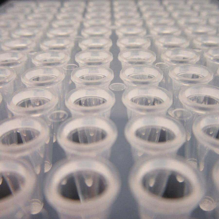
• Batch SAXS: a small volume of sample (~30 microliters) is loaded into a flow cell in a vacuum box and oscillated during X-ray exposure. Requires pure, monodisperse sample and a precisely matching buffer measurement for subtraction.
Sample preparation
- Sample quality:
Samples should be monodisperse and at a high enough concentration (see next section for details). For batch SAXS, it is a good idea to bring at least some unconcentrated sample to test for concentration-induced aggregation. You should check monodispersity using dynamic light scattering (DLS), if available. Purifying by size-exclusion chromatography is highly recommended, though sometimes, pure proteins will aggregate rapidly afterwards. It may be necessary to test different conditions under which the protein is monodisperse and well behaved. Protein samples have been frozen successfully for shipment, but users should not assume their proteins will freeze-thaw well.
- Buffer additives:
A small amount of glycerol (1 - 5%) is advisable for protection from radiation damage, but more than 15% will degrade the strength of your scattering signal and should be avoided. In general, high salt (> 1 M) should be avoided for the same reason. Additives like DTT and TCEP are known to reduce radiation damage in small amounts and helpful to include.
Additional considerations for batch SAXS
- Provide a precisely matched buffer solution for background subtraction:
This should be the exact same buffer as in the sample. Buffer exchange (by centrifugal concentrator, dialysis, or SEC) if needed. Prepare plenty of extra buffer for sample dilutions and for rinsing sample cells (bring at least 10 ml if you can).
- Measure your concentration as accurately as possible:
Molecular weight estimates based on known concentrations are valuable indicators of sample monodispersity, oligomeric state, and can help diagnose problems with mixtures. A280 measurements can be conducted in the S7 chemistry lab.
- Sample volumes:
Individual exposures can be done with sample volumes as small as 20 microliters if loaded by hand. But for easy and reliable sample loading, we recommend using the sample loading robot with at least 30 microliters. Larger sample volumes ensure easy and rapid positioning of sample in the beam and a generous oscillation size, which will eliminate potential radiation damage.
Since BioSAXS requires multiple dilutions to check for concentration effects, it is advisable to bring more than the minimum volume. A sample size of 50 microliters, for example, would allow just enough to prepare a minimum series of 3 dilutions of 30 microliters each: full strength (30 ul sample), 66% (20 ul sample + 10 ul buffer), and 33% (10 ul sample + 20 ul buffer). More dilutions are desirable. Many users prefer to prepare dilutions by halving: 1.0, 0.5, 0.25 0.125 etc.
Collecting data at several (at least 3) different concentrations will allow you to extrapolate to infinite dilution if necessary. Alternatively, you can combine a dilute curve (small-angle part) with a concentrated curve (wide-angle part). Concentration does not affect the wide angle part of the scattering curve.
What sample concentrations do I need?
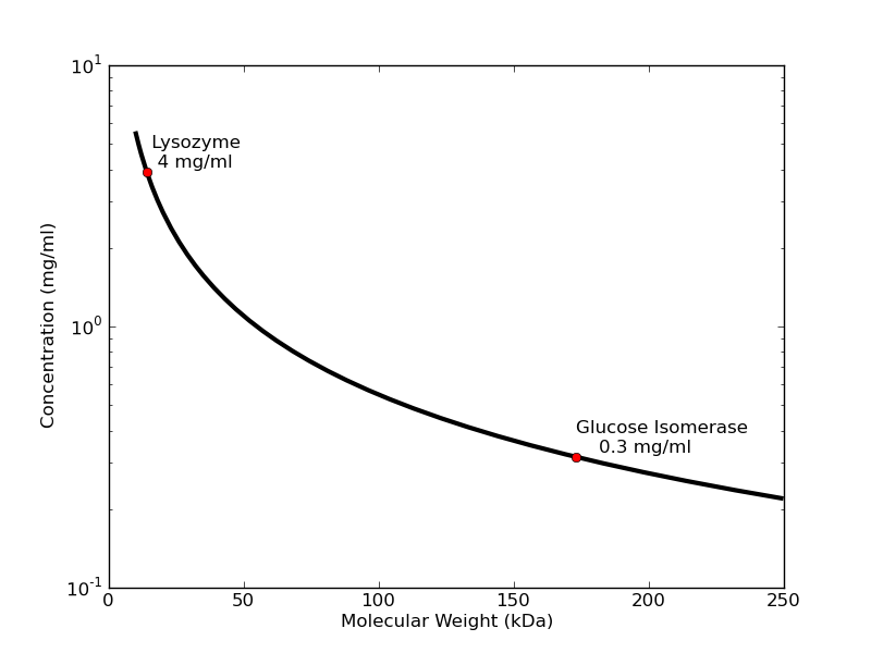
The concentration of protein necessary to get a good signal depends inversely on molecular weight. For small proteins like lysozyme collected on S7A station using typical exposure times, 4 mg/ml will usually produce a profile that is dilute enough to avoid interparticle interactions, but strong enough to give a good low-noise Guinier plot with accurate radius of gyration. Larger proteins like glucose isomerase (173 kDa) need only 0.3 mg/ml to give the same strength of signal in the low-angle region. Note that when solutions are too concentrated, samples may exhibit concentration-related distortions in the small-angle part of the scattering profile. You can see this in lysozyme samples >10 mg/ml and glucose isomerase >0.5 mg/ml.
A good rule of thumb for "dilute" sample concentration is 60/(molecular weight in kDa) = concentration (mg/ml). Best to bring more concentrated sample (× 5) so you can create a concentration series, as dilutions are cheap. Generally, SEC-SAXS requires 100 microliters of sample at 5×60/(molecular weight) mg/mL (for a 10/300 column. A 5/150 column will dilute less and can handle ~50 microliters).
How many samples to bring?
- Batch SAXS
Expect to measure approximately 80 samples in the first 24 hours. Experienced users may collect far more. As of Fall 2024, our sample loading robot can load one sample and clean a flow cell in ~5 minutes total.
Actual time for data collection is hard to estimate because there are many variables. Currently, we are recommending at least ten 1 second exposures per sample, so the total exposure would be 10 seconds. Each protein you examine will include a buffer exposure of equal length and at least 3 concentrations. You may use the same buffer profile for multiple proteins, if you like. But, it is *very* wise to re-take the buffer periodically (every 4 samples or so) as the capillary background can change slowly with use. You may wish to expose dilute solutions for longer using larger sample volumes. Spinning samples prior to data collection requires 5-10 min at 14,000 rpm, but can be done simultaneously with data collection.
- SEC-SAXS
Superdex Increase 5/150 column (good for cleanup of samples and removal of aggregation): at least 25 samples in 24 hours, if there are no buffer changes. For every buffer change, subtract 2 samples (i.e., 2 column volumes).
Superdex Increase 10/300 column (higher resolution): roughly twice as long, at ~50 minutes for the 23 mL column. Actual performance will vary widely. With experience and teamwork, sample throughput can be significantly higher.
Potential problems
- aggregation (most common)
- molecule too large (beamline can't reach low enough q)
- sample is a mixture (common with complexes)1
- sample too dilute
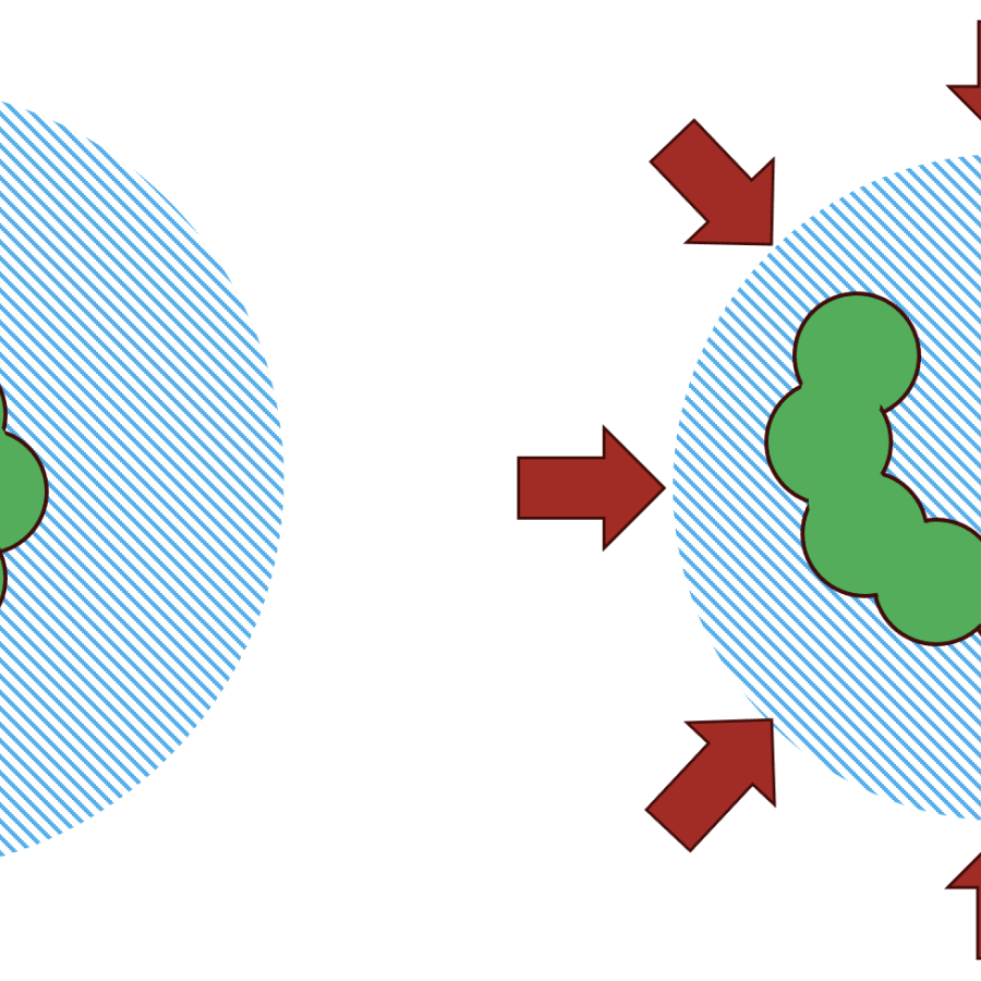
- radiation damage
- denaturation (rare)
- buffer mismatch
- contrast problems (weak signal due to buffer composition)
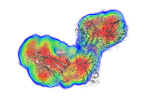
- heterogeneous sample (protein-DNA-lipid complexes)2
1Generally, solutions must be pure and monodisperse for standard SAXS analysis to work. If you are hoping to see a conformational change when you add a component like a small ligand or other binding partner to the protein sample, be careful to maintain exactly matching buffer. This may mean changing buffer again using a centrifugal concentrator, dialysis, or a SEC run. If conversion of your protein to the new state is incomplete, you may need to re-purify. Mixtures can be treated with BioSAXS, but this is an advanced topic and additional information and multiple experiments may be required to understand the data.
2Mixed complexes of protein, DNA, and/or lipids can cause problems with certain SAXS calculations.
Protein standards
MacCHESS provides several protein standards for use in your SAXS experiments. It is important to run at least one standard so that 1) you have a way to estimate molecular mass and 2) you can be confident that the beamline is running properly. Standards also serve as a reminder of what good monodisperse sample *should* look like.
Lysozyme Buffer:
40 mM NaOAc, pH 4.0
150 mM NaCl
1% glycerol (v/v)
Glucose Isomerase Buffer:
10 mM HEPES, pH 7.0
1 mM MgCl2
Protein concentrations vary from run to run, but approximately 4 mg/ml for lysozyme and 0.4 mg/ml for glucose isomerase work well. A more complete list of standards can be found in:
Mylonas E, Svergun DI. "Accuracy of molecular mass determination of proteins in solution by small-angle X-ray scattering", J. Appl. Cryst. 40:S245-S249 (2007).
Kozak M. "Glucose isomerase from Streptomyces rubiginosus - potential molecular weight standard for small-angle X-ray scattering." J. Appl. Cryst. 38:555-558 (2005).
Temperature control
| Method | Temperature range |
| Batch | 4 °C to 80 °C |
| SEC-SAXS | 4 °C and ambient temperature (~28 °C) |
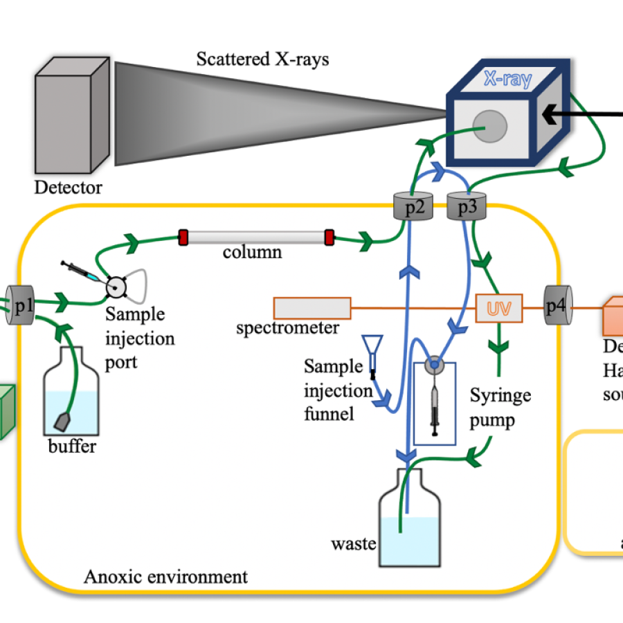
| Anoxic SAXS | 4 °C and ambient temperature (~28 °C) |
| HP-SAXS | 4 °C to 80 °C |
| HP-SEC-SAXS | 4 °C to 50 °C |
We have calibrated the actual sample temperature using a micro thermocouple and provide a correction table for setting the chiller for normal BioSAXS operation (courtesy of Matt McLeod): CHESS_7A1_temperature_0.xls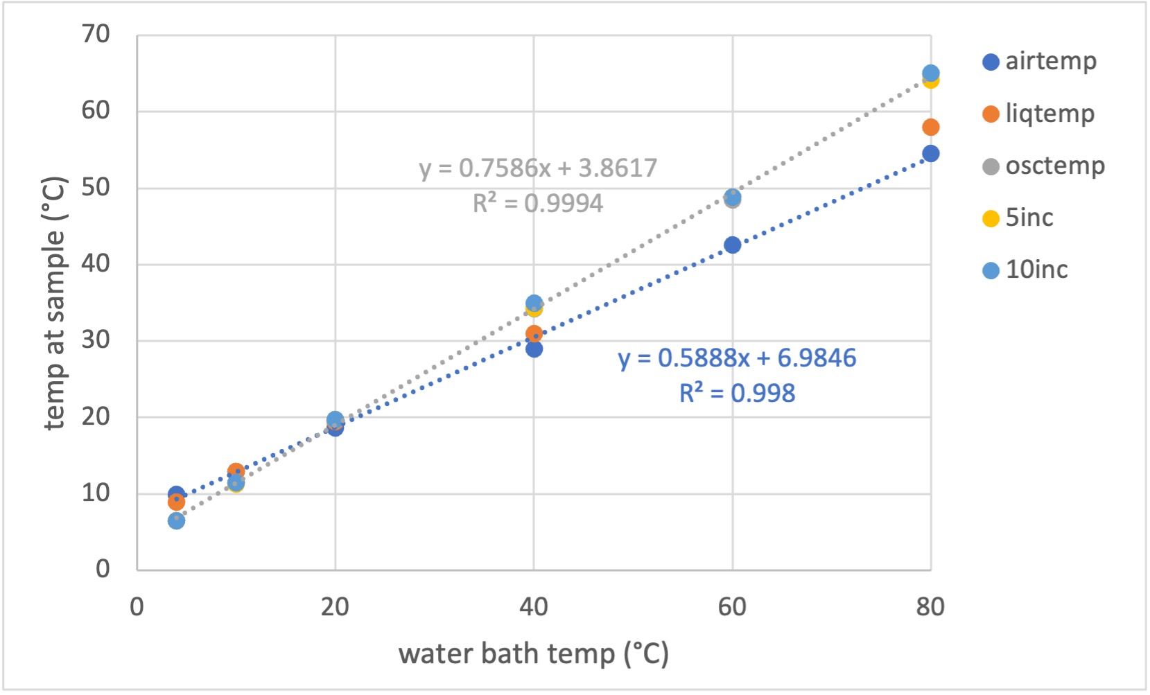
Legend explanation:
• airtemp: air temperature
• liqtemp: temperature of liquid in the capillary. Not oscillating and not incubated in the block.
• osctemp: oscillating liquid plug - this takes less than a minute to get to temperature. As it moves into the capillary, the sample heats significantly and needs a little more time to get fully equilibrated.
• 5inc and 10inc: 5 and 10 minute incubation in the block, followed by moving sample into the capillary for temperature measurement. If not oscillating, the temperature steadily goes down to "liquid" temperature.
Understanding exposure time, dose, and normalization
Collecting data with spec
When you use the spec command rgseries <number of snapshots> <exposure time per snapshot>, the X-ray shutter will open and the detector will take the designated number of images with no delay in between. Each image will accumulate photons for "exposure time per snapshot" seconds. When finished, the shutter will close. For batch SAXS experiments, the sample will be exposed to X-rays for a total of "(number of snapshots)×(time per snapshot)" seconds. Longer exposure times or more snapshots will increase the total dose. This can improve the signal strength, but also risk more X-ray damage. Finding the appropriate total dose is a matter of experimentation, but your beamline scientist will start you with recommended settings based on common proteins.
For SEC-SAXS, images are also acquired continuously over the duration of the experiment. For example, rgseries 1500 2, will collect 1500 2-second exposure frames. Changing the exposure time does not affect the dose because the shutter is open the entire time, irradiating the eluate as it leaves the SEC. To reduce damage, the beam can be attenuated, the flow increased, or rgseries_pauses can add dark periods (the shutter is closed for a specified time between exposures). The beamline scientists can help adjust your experiment as needed.
Data processing on BioXTAS RAW
When RAW reads a detector image, it applies a normalization factor based on the integrated transmitted intensity. As a consequence, scattering profiles taken at different exposure times and different attenuations will overlay (reasonably well). Normalization is applied because synchrotron beams can fluctuate in intensity over time (during top-offs, for example). So, normalization allows you to compensate for slight differences in sample dose. It is not intended to compensate for large changes that might result from intentional attenuation. So, it is always recommended to subtract like exposures with like exposures, when possible.
Finally, RAW usually applies a scaling factor to place the scattering profile on an absolute scale. As a consequence of how normalization is performed, scattering profiles will always be on an absolute scale regardless of exposure time or incident beam intensity. Setting absolute scale with water
It is important at the start of any visit to verify all of the above settings in the RAW software and save the appropriate .cfg file containing those settings.